 [click]
|
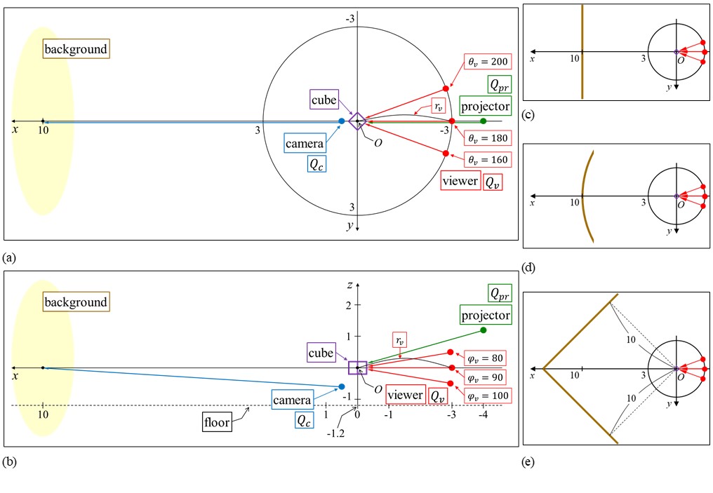
Position [r, θ, φ] (r: meters) (θ, φ: degrees) |
Position [x, y, z] (meters) |
Gaze point [x, y, z] (meters) |
Angles of view [αx, αy] (degrees) |
Numbers of pixels [Mx, My] |
|
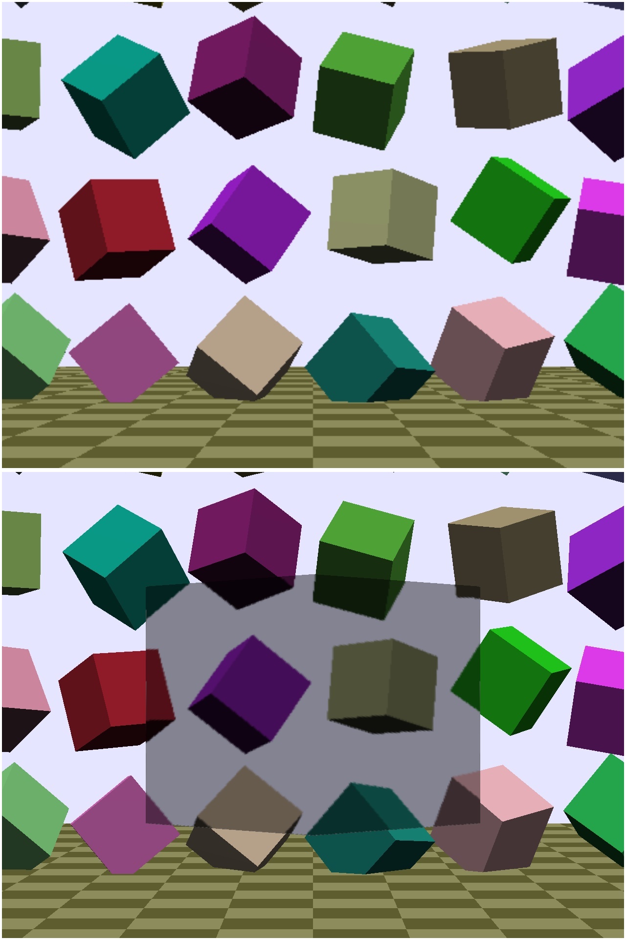
| Viewer: Qvini | 3.0, 180.0, 90.0 | -3.0, 0.0, 0.0 | 0.0, 0.0, 0.0 | 20.0, 15.0 | 640, 480 |
| Projector: Qpr | 4.2, 180.0, 74.0 | -4.0, 0.0, 1.2 | 0.0, 0.0, 0.0 | 38.0, 23.0 | 640, 400 |
| Camera: Qc | 0.8, 0.0, 140.0 | 0.5, 0.0, -0.6 | 10.0, 0.0, 0.0 | 57.0, 43.0 | 640, 480 |
 [click]
 [click]
 [click]
 [click]
 [click]
 [click]
 [click]
 [click]
 [click]
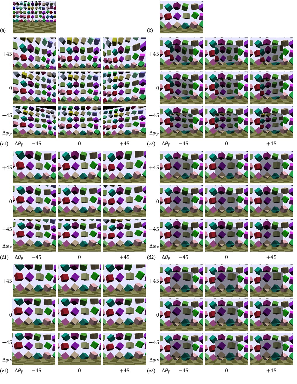
| LPG | ΔθPG | ΔφPG | |
| (a) | 10.0 | 0.0 | 0.0 |
| (b) | 10.0 | 0.0 | 0.0 |
| Minimum coordinate | Maximum coordinate | Number of points | Interval | |
| ri | rmin = 2.5 | rmax = 3.5 | Nr = 3 | Δr = 0.5 |
| θj | θmin = 0 | θmax = 360 | Nθ = 18 | Δθ = 20 |
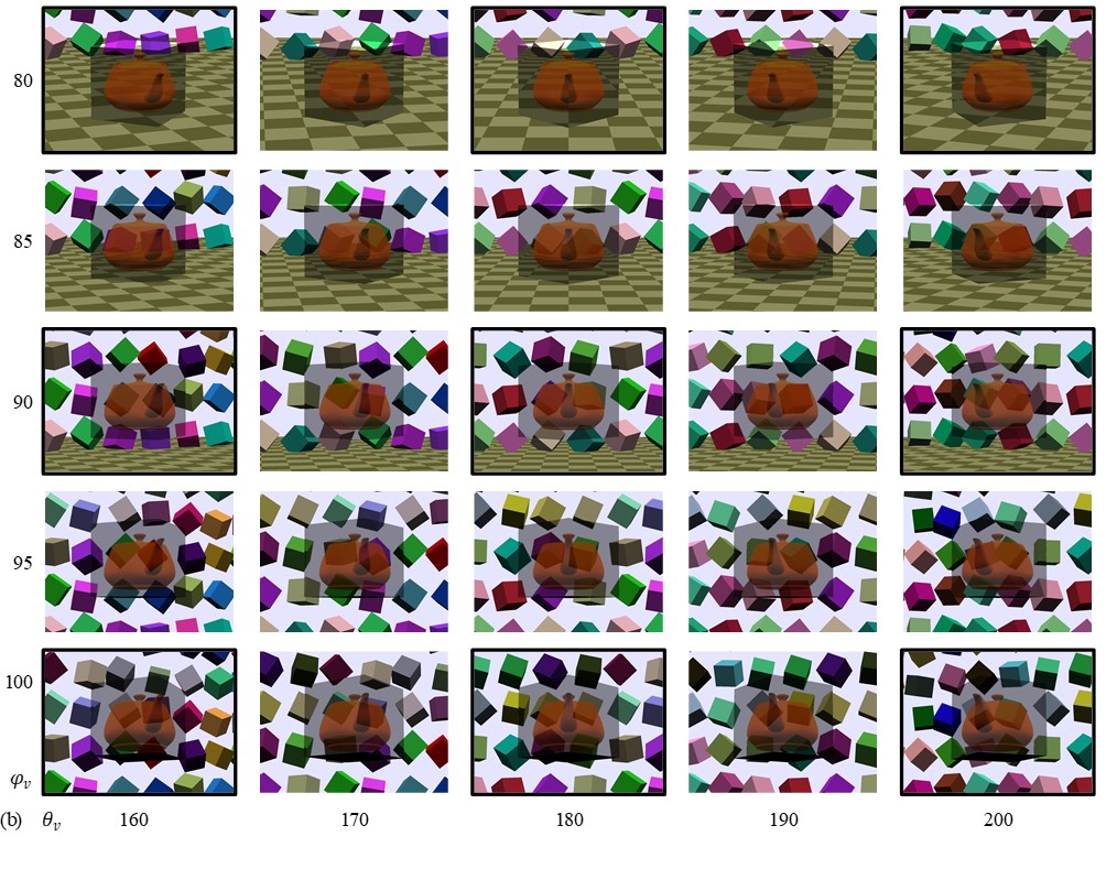
| φk | φmin = 80 | φmax = 100 | Nφ = 3 | Δφ = 10 |
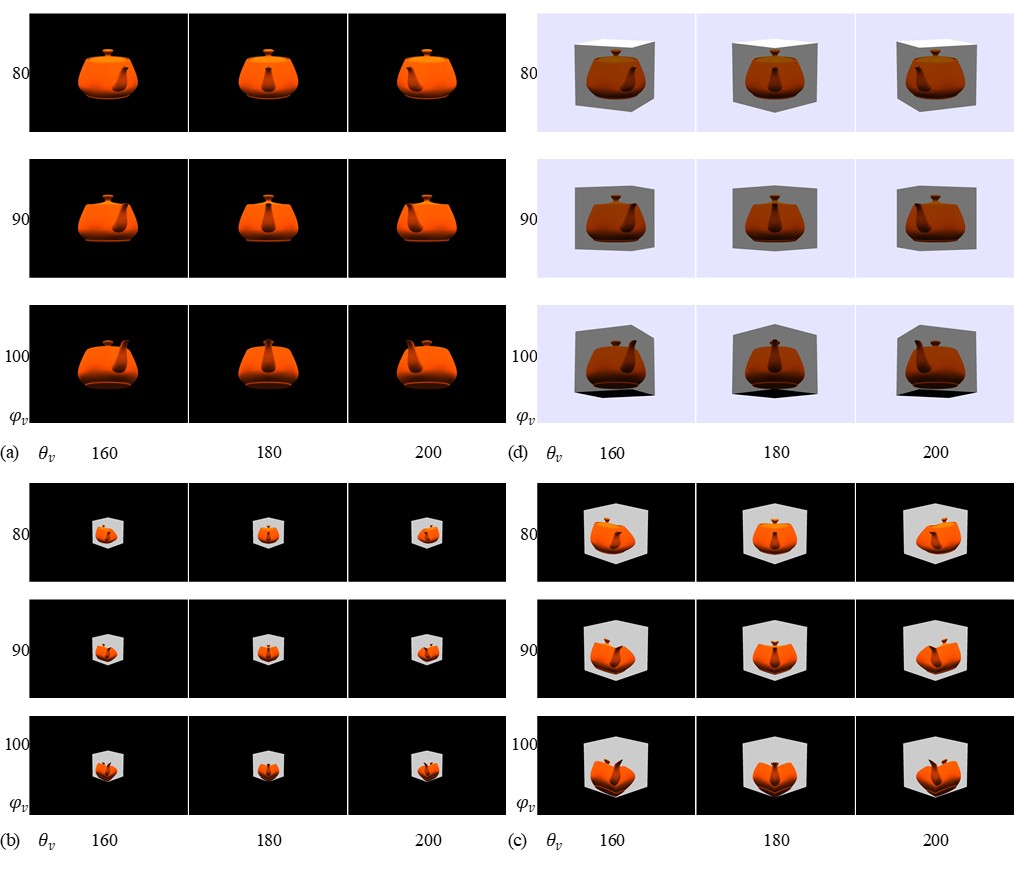
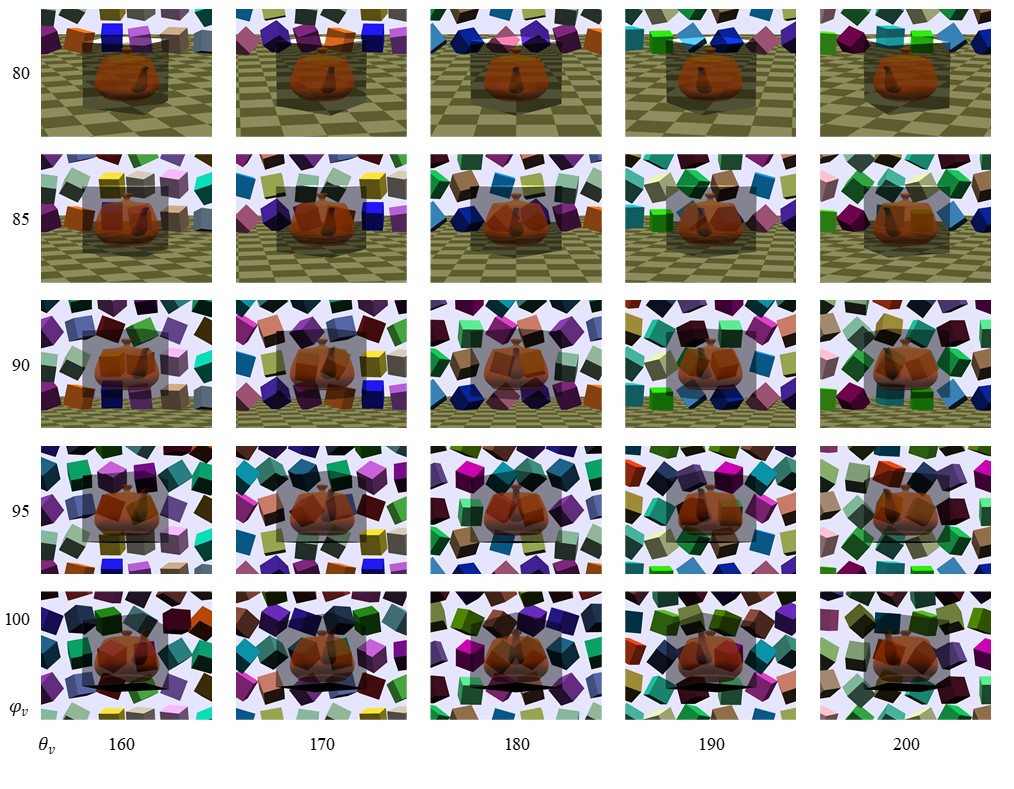
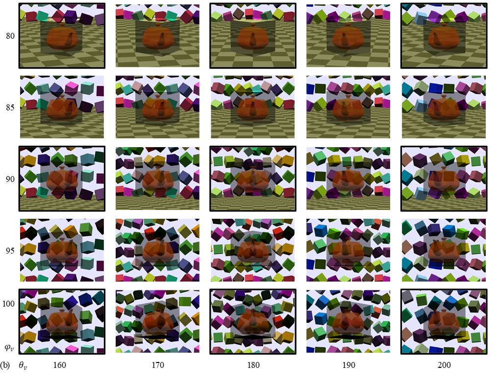
| ri | 3.0 | ||||||||
| θj | 160 | 180 | 200 | ||||||
| φk | LPL | ΔθPL | ΔφPL | LPL | ΔθPL | ΔφPL | LPL | ΔθPL | ΔφPL |
| 80 | 0.805944 | 20.0 | -10.0 | 0.154266 | 0.0 | -10.0 | 0.805944 | -20.0 | -10.0 |
| 90 | 0.641778 | 20.0 | 0.0 | 0.0 | 0.0 | 0.0 | 0.641778 | -20.0 | 0.0 |
| 100 | 0.805944 | 20.0 | 10.0 | 0.154266 | 0.0 | 10.0 | 0.805944 | -20.0 | 10.0 |
 [click]
 [click]
 [click]
 [click]
 [click]
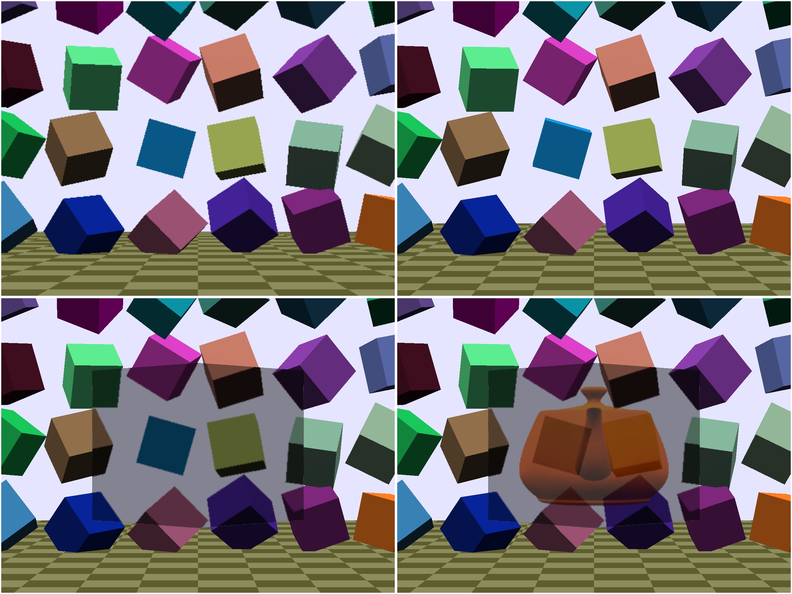
| LPG | ΔθPG | ΔφPG | |
| (a) | 12.8 | 0.0 | 0.0 |
| (b) | 10.0 | 0.0 | 0.0 |
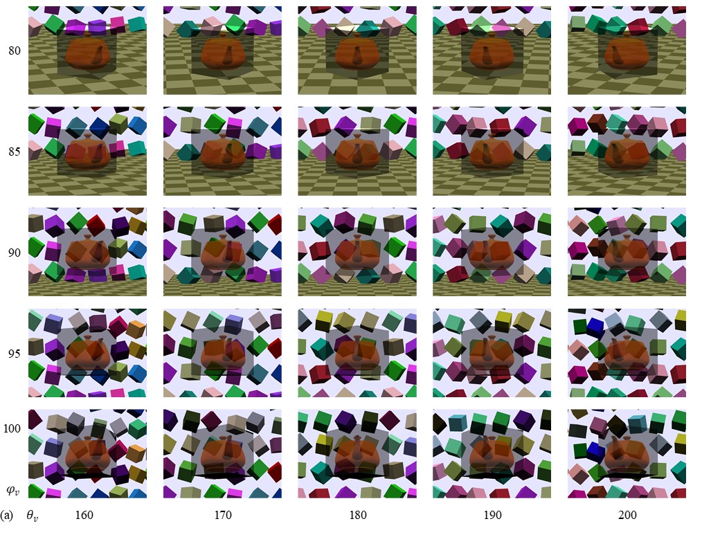
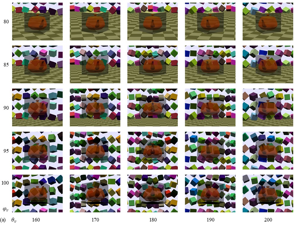
| ri | 3.0 | ||||||||
| θj | 160 | 180 | 200 | ||||||
| φk | LPL | ΔθPL | ΔφPL | LPL | ΔθPL | ΔφPL | LPL | ΔθPL | ΔφPL |
| 80 | 1.203993 | -25.0 | -10.0 | 2.997460 | 0.0 | -10.0 | 1.203993 | 25.0 | -10.0 |
| 90 | 1.033779 | -25.0 | 0.0 | 2.8 | 0.0 | 0.0 | 1.033779 | 25.0 | 0.0 |
| 100 | 1.203993 | -25.0 | 10.0 | 2.997460 | 0.0 | 10.0 | 1.203993 | 25.0 | 10.0 |
 [click]
 [click]
 [click]
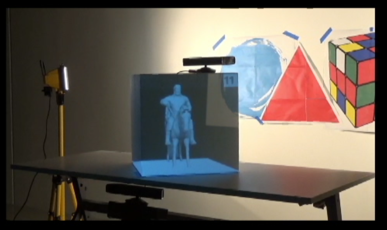
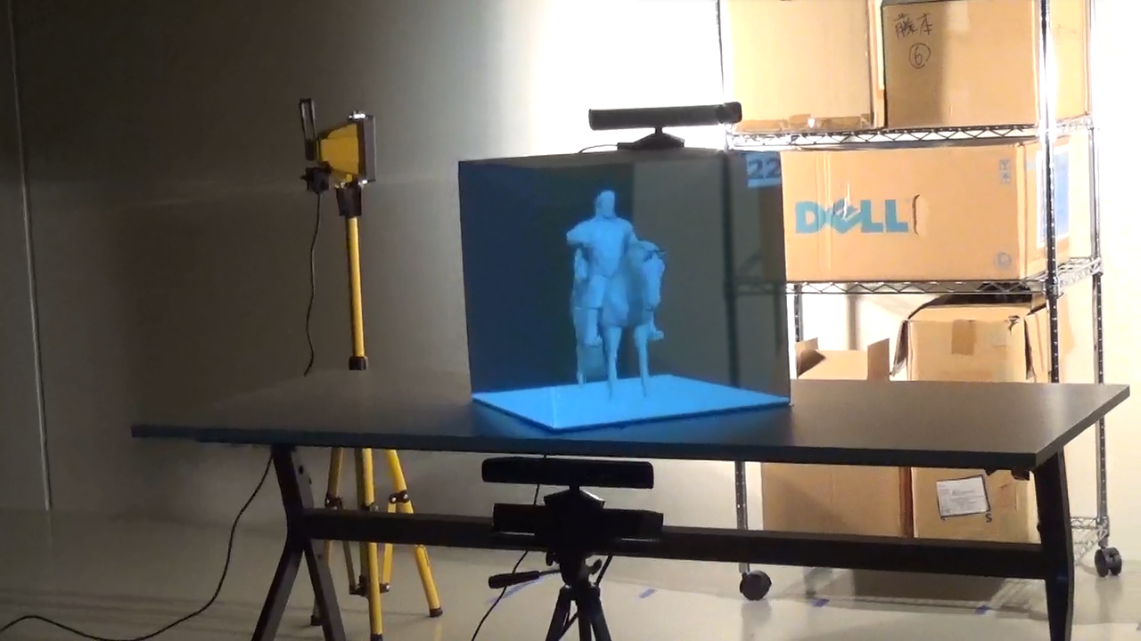
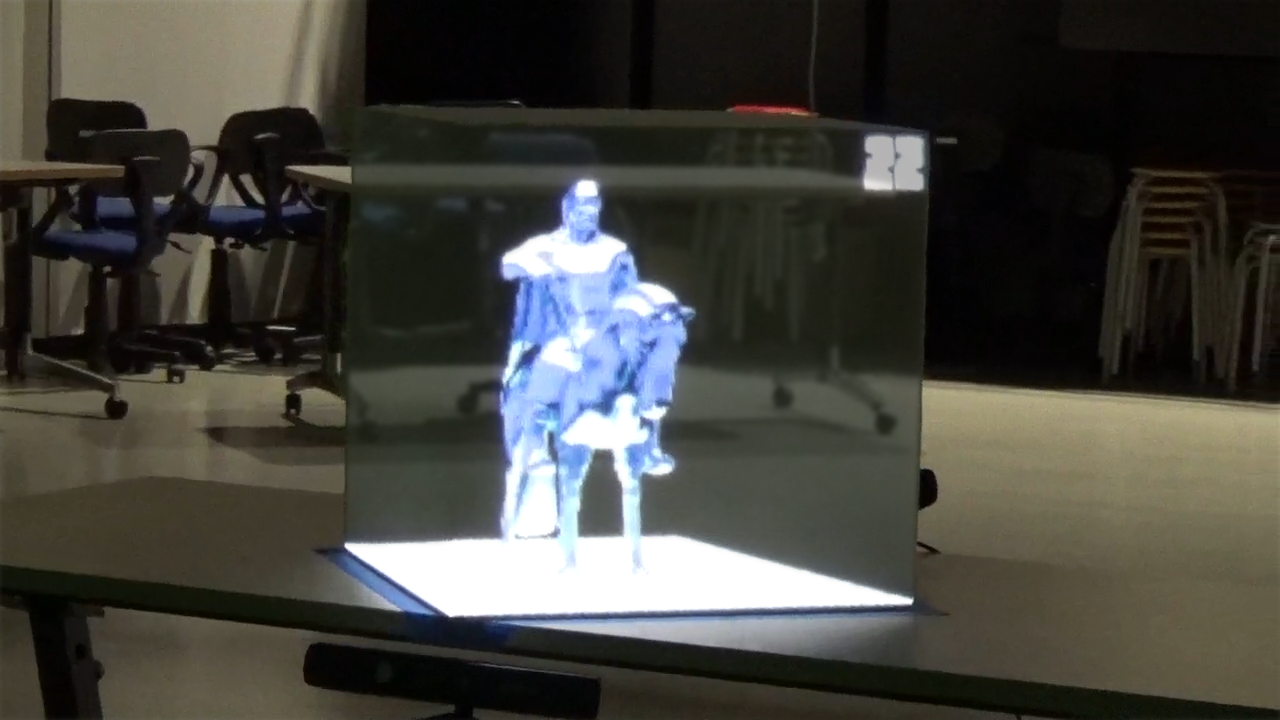
| Projector | RICOH IPSiO PJ WX5150 |
| Tracking sensor | Kinect for Windows |
| Camera | Kinect for Windows |
| Personal computer | OS: Windows 10, Chipset: Intel(R) Z370 Express, CPU: Intel(R) Core i7-8700K (3.7-4.7GHz), GPU: NVIDIA(R) GeForce GTX 1060 6GB GDDR5, Mem: 32GB, SSD: 480GB, HDD: 2TB. |
 [click]
 [click]
 [click]
 [click]